
#computerscience #cpp #python #productivity
Data Structures & Algorithms (DSA) is often considered to be an intimidating topic - a common misbelief. Forming the foundation of the most innovative concepts in tech, they are essential in both jobs/internships applicants' and experienced programmers' journey. Mastering DSA implies that you are able to use your computational and algorithmic thinking in order to solve never-before-seen problems and contribute to any tech company's value (including your own!). By understanding them, you can improve the maintainability, extensibility and efficiency of your code.
This article is aiming to make DSA not look as intimidating as it is believed to be. It includes the 15 most useful data structures and the 15 most important algorithms that can help you ace your interviews and improve your competitive programming skills. Each chapter includes useful links with additional information and practice problems. DS topics are accompanied by a graphic representation and key information. Every algorithm is implemented into a continuously updating Github repo. At the time of writing, it contains the pseudocode, C++, Python and Java (still in progress) implementations of each mentioned algorithm (and not only). This repository is expanding thanks to other talented and passionate developers that are contributing to it by adding new algorithms and new programming languages implementations.
Contents
I. Data Structures
Arrays
Linked Lists
Stacks
Queues
Maps & Hash Tables
Graphs
Trees
Binary Trees & Binary Search Trees
Self-balancing Trees (AVL Trees, Red-Black Trees, Splay Trees)
Heaps
Tries
Segment Trees
Fenwick Trees
Disjoint Set Union
Minimum Spanning Trees
II. Algorithms
Divide and Conquer
Sorting Algorithms (Bubble Sort, Counting Sort, Quick Sort, Merge Sort, Radix Sort)
Searching Algorithms (Linear Search, Binary Search)
Sieve of Eratosthenes
Knuth-Morris-Pratt Algorithm
Greedy I (Maximum number of non-overlapping intervals on an axis)
Greedy II (Fractional Knapsack Problem)
Dynamic Programming I (0–1 Knapsack Problem)
Dynamic Programming II (Longest Common Subsequence)
Dynamic Programming III (Longest Increasing Subsequence)
Convex Hull
Graph Traversals (Breadth-First Search, Depth-First Search)
Floyd-Warshall / Roy-Floyd Algorithm
Dijkstra's Algorithm & Bellman-Ford Algorithm
Topological Sorting
I. Data Structures
1. Arrays
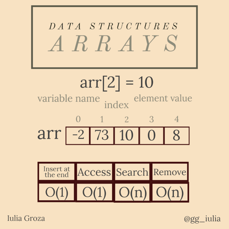
Arrays are the simplest and most common data structures. They are characterised by the facile access of elements by index (position).
What are they used for?
Imagine having a theater chair row. Each chair has assigned a position (from left to right), therefore every spectator will have assigned the number from the chair (s)he will be sitting on. This is an array. Expand the problem to the whole theater (rows and columns of chairs) and you will have a 2D array (matrix)!
Properties
elements' values are placed in order and accessed by their index from 0 to the length of the array-1;
an array is a continuous block of memory;
they are usually made of elements of the same type (it depends on the programming language);
access and addition of elements are fast; search and deletion are not done in O(1).
Useful Links
GeeksforGeeks: Introduction to arrays
2. Linked Lists
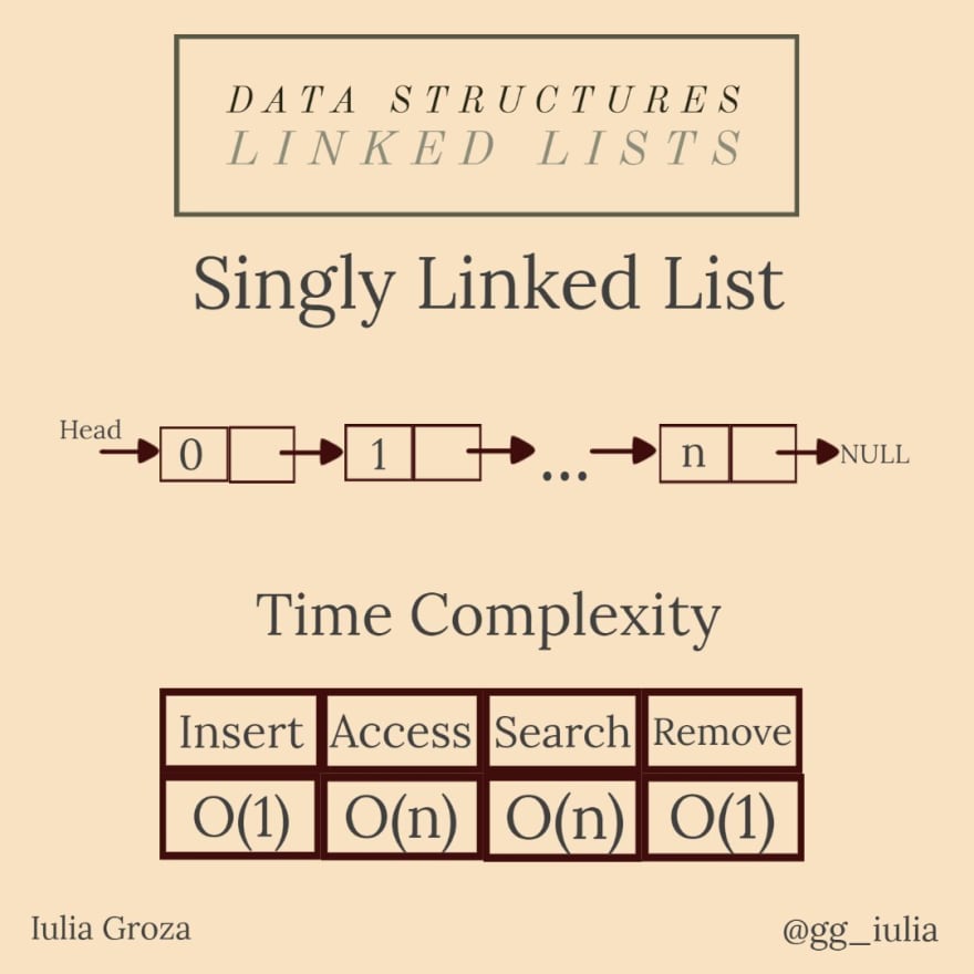
Linked lists are linear data structures, just like arrays. The main difference between linked lists and arrays is that elements of a linked list are not stored at contiguous memory locations. It is composed of nodes - entities that store the current element's value and an address reference to the next element. That way, elements are linked by pointers.
What are they used for?
One relevant application of linked lists is the implementation of the previous and the next page of a browser. A double linked list is the perfect data structure to store the pages displayed by a user's search.
Properties
they come in three types: singly, doubly and circular;
elements are NOT stored in a contiguous block of memory;
perfect for an excellent memory management (using pointers implies dynamic memory usage);
insertion and deletion are fast; accessing and searching elements are done in linear time.
Useful Links
3. Stacks
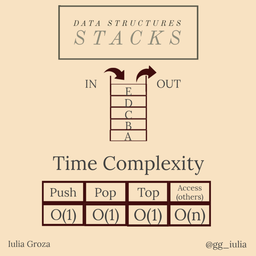
A stack is an abstract data type that formalizes the concept of restricted access collection. The restriction follows the rule LIFO (Last In, First Out). Therefore, the last element added in the stack is the first element you remove from it.
Stacks can be implemented using arrays or linked lists.
What are they used for?
The most common real-life example uses plates placed one over another in the canteen. The plate which is at the top is the first to be removed. The plate placed at the bottommost is the one that remains in the stack for the longest period of time.
One situation when stacks are the most useful is when you need to obtain the reverse order of given elements. Just push them all in a stack and then pop them.
Another interesting application is the Valid Parentheses Problem. Given a string of parantheses, you can check that they are matched using a stack.
Properties
you can only access the last element at one time (the one at the top);
one disadvantage is that once you pop elements from the top in order to access other elements, their values will be lost from the stack's memory;
access of other elements is done in linear time; any other operation is in O(1).
Useful Links
CS Academy: Stack Introduction
CS Academy: Stack Application - Soldiers Row
4. Queues
A queue is another data type from the restricted access collection, just like the previously discussed stack. The main difference is that the queue is organised after the FIFO (First In, First Out) model: the first inserted element in the queue is the first element to be removed. Queues can be implemented using a fixed length array, a circular array or a linked list.
What are they used for?
The best use of this abstract data type (ADT) is, of course, the simulation of a real life queue. For example, in a call center application, a queue is used for saving the clients that are waiting to receive help from the consultant - these clients should get help in the order they called.
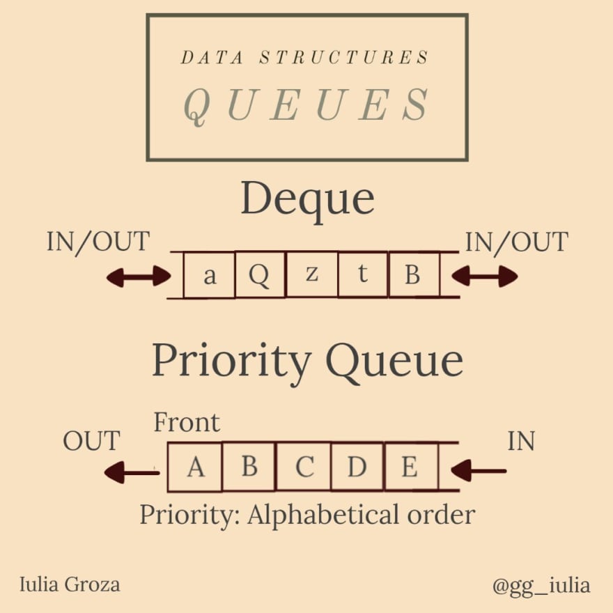
One special and very important type of queue is the priority queue. The elements are introduced in the queue based on a "priority" associated with them: the element with the highest priority is the first introduced in the queue. This ADT is essential in many Graph Algorithms (Dijkstra's Algorithm, BFS, Prim's Algorithm, Huffman Coding - more about them below). It is implemented using a heap.
Another special type of queue is the deque (pun alert it's pronounced "deck"). Elements can be inserted/removed from both endings of the queue.
Properties
we can directly access only the "oldest" element introduced;
searching elements will remove all the accessed elements from the queue's memory;
popping/pushing elements or getting the front of the queue is done in constant time. Searching is linear.
Useful Links
5. Maps & Hash Tables
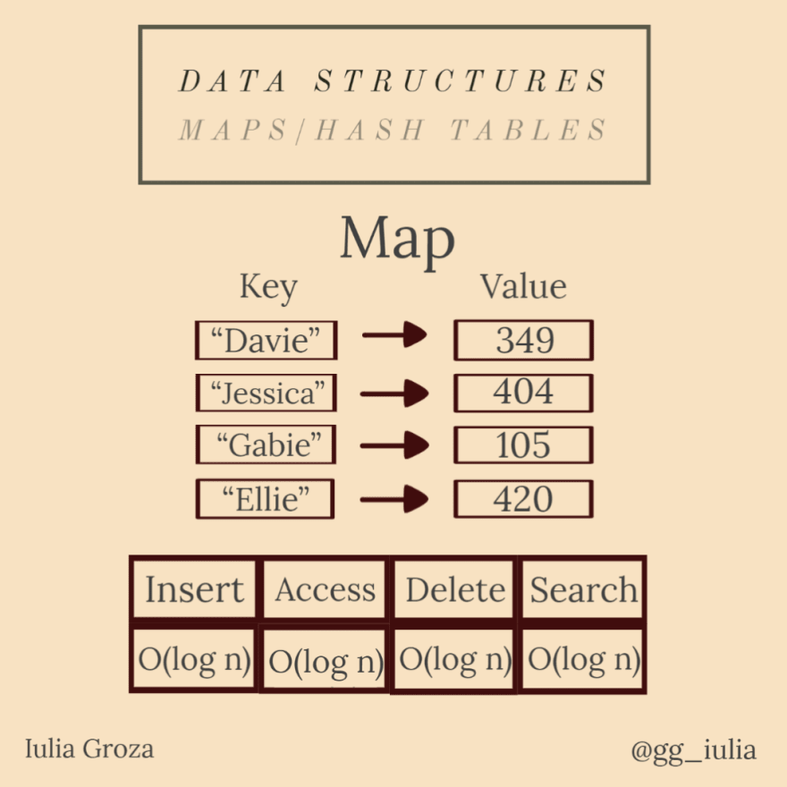
Maps (dictionaries) are abstract data types that contain a collection of keys and a collection of values. Each key has a value associated with it.
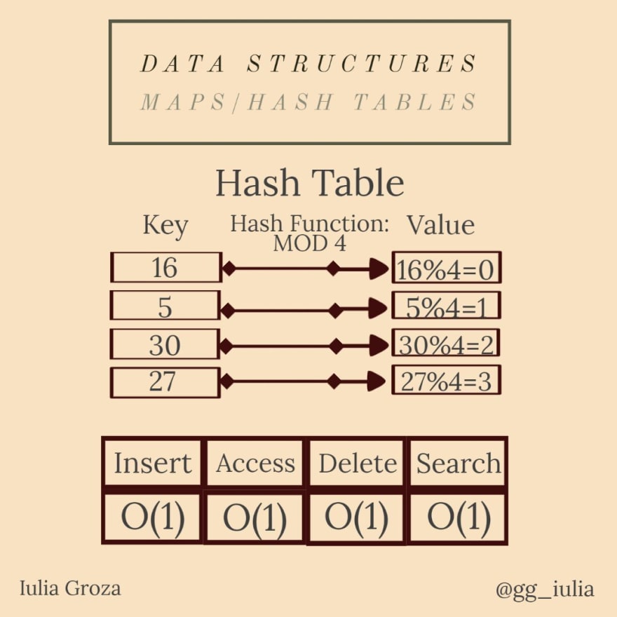
A hash table is a particular type of map. It uses a hash function to generate a hash code, into an array of buckets or slots: the key is hashed and the resulting hash indicates where the value is stored.
The most common hash function (among many) is the modulo constant function. e. g. if the constant is 6, the value of the key x is x%6.
Ideally, a hash function will assign each key to a unique bucket, but most of their designs employ an imperfect function, which might conduct to collision between keys with the same generated value. Such collisions are always accomodated in some way.
What are they used for?
The most known application of maps is a language dictionary. Each word from a language has assigned its definition to it. It is implemented using an ordered map (its keys are alphabetically ordered).
Contacts is also a map. Each name has a phone number assigned to it.
Another useful application is normalization of values. Let's say we want to assign to each minute of a day (24 hours = 1440 minutes) an index from 0 to 1439. The hash function will be h(x) = x.hour*60+x.minute.
Properties
keys are unique (no duplicates);
collision resistance: it should be hard to find two different inputs with the same key;
pre-image resistance: given a value H, it should be hard to find a key x, such that h(x)=H;
second pre-image resistance: given a key and its value, it should be hard to find another key with the same value;
terminology:
* "map": Java, C++;
* "dictionary": Python, JavaScript, .NET;
* "associative array": PHP.
because maps are implemented using self-balancing red-black trees (explained below), all operations are done in O(log n); all hash table operations are constant.
Useful Links
6. Graphs
A graph is a non-linear data structure representing a pair of two sets: G={V, E}, where V is the set of vertices (nodes), and E the set of edges (arrows). Nodes are values interconnected by edges - lines that depict the dependency (sometimes associated with a cost/distance) between two nodes.
There are two main types of graphs: directed and undirected. In an undirected graph, the edge (x, y) is available in both directions: (x, y) and (y, x). In a directed graph, the edge (x, y) is called an arrow and the direction is given by the order of the vertices in its name: arrow (x, y) is different from arrow (y, x).
What are they used for?
Graphs are the foundation of every type of network: a social network (like Facebook, LinkedIn), or even the network of streets from a city. Every user of a social media platform is a structure containing all of his/her personal data - it represents a node of the network. Friendships on Facebook are edges in an undirected graph (because it is reciprocal), while on Instagram or Twitter, the relationship between an account and its followers/following accounts are arrows in a directed graph (not reciprocal).
Properties
Graph theory is a vast domain, but we are going to highlight a few of the most known concepts:
the degree of a node in an undirected graph is the number of its incident edges;
the internal/external degree of a node in a directed graph is the number of arrows that direct to/from that node;
a chain from node x to node y is a succesion of adjacent edges, with x as its left extremity and y as its right;
a cycle is a chain were x=y; a graph can be cyclic/acyclic; a graph is connected if there is a chain between any two nodes from V;
a graph can be traversed and processed using Breadth First Search (BFS) or Depth First Search (DFS), both done in O(|V|+|E|), where |S| is the cardinal of the set S; Check the links below for other essential info in graph theory.
Useful Links
Wikipedia: Graphs - Discrete Mathematics
CS Academy: Graph representation
7. Trees
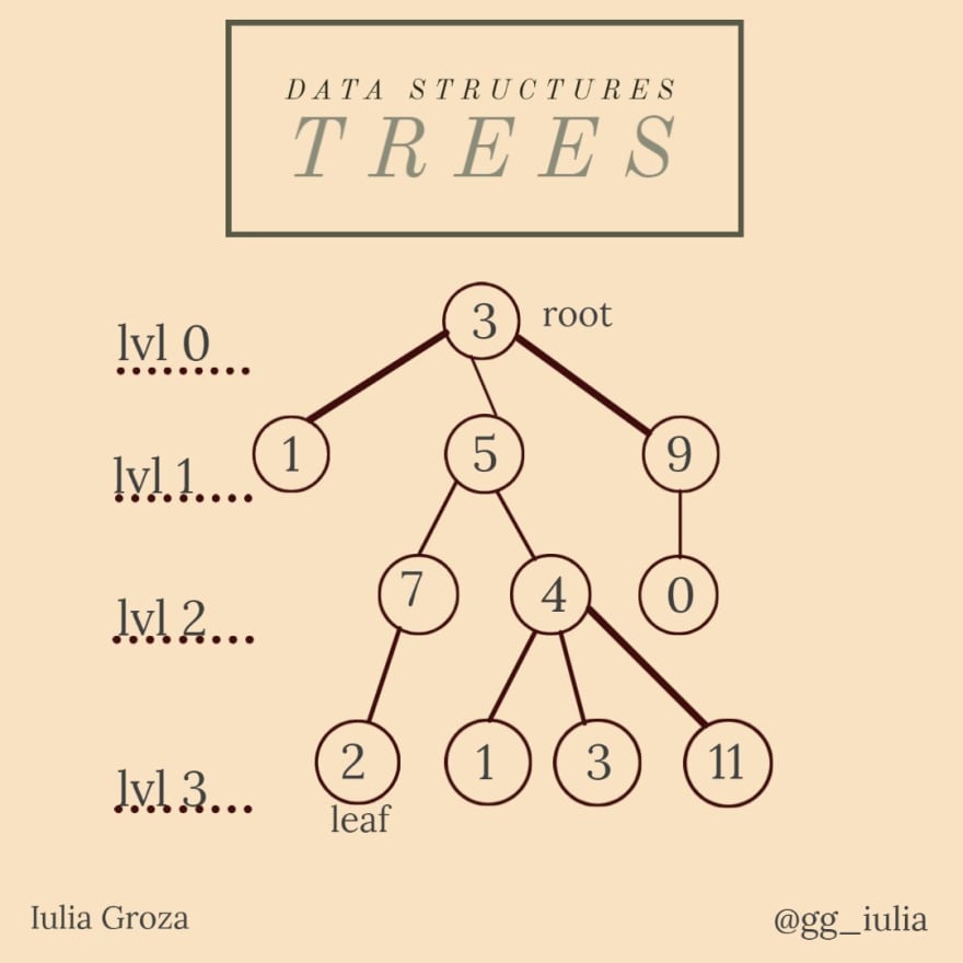
A tree is an undirected graph, minimal in terms of connectivity (if we eliminate a single edge the graph won't be connected anymore) and maximal in terms of acyclicity (if we add a single edge the graph won't be acyclic anymore). So any acyclic connected undirected graph is a tree, but for simplicity, we will refer to rooted trees as trees.
A root is one fixed node that establishes the direction of the edges in the tree, so that's where everything "starts". Leaves are the terminal nodes of the tree - that's where everything "ends".
A child of a vertice is its incident vertice below it. A vertice can have multiple children. A vertice's parent is its incident vertice above it - it's unique.
What are they used for?
We use trees anytime we should depict a hierarchy. Our own genealogical tree is the perfect example. Your oldest ancestor is the root of the tree. The youngest generation represents the leaves' set.
Trees can also represent the subordinate relationship in the company you work for. That way you can find out who is your manager and who you should manage.
Properties
the root has no parent;
leaves have no children;
the length of the chain between the root and a node x represents the level x is situated on;
the height of a tree is the maximum level of it (3 in our example);
the most common method to traverse a tree is DFS in O(|V|+|E|), but we can use BFS too; the order of the nodes traversed in any graph using DFS form the DFS tree that indicates us the time a node has been visited.
Useful Links
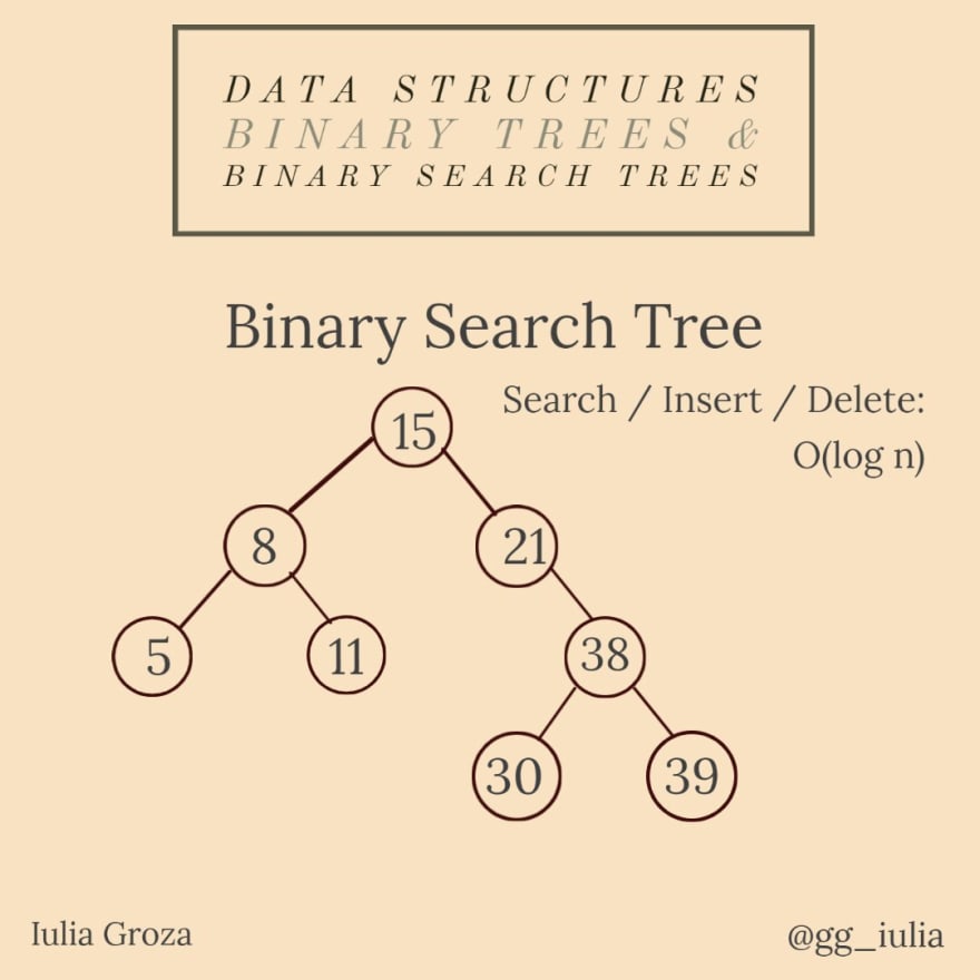
8. Binary Trees & Binary Search Trees
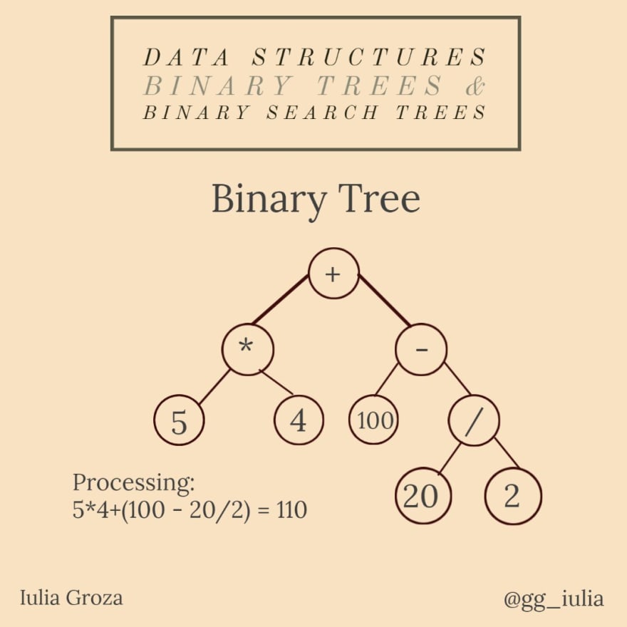
A Binary Tree is a special type of tree: each vertice can have maximum two children. In a strict binary tree, every node has exactly two children, except for the leaves. A complete binary tree with n levels has all 2ⁿ-1 possible nodes.
A binary search tree is a binary tree where nodes' values belong to a totally ordered set - any arbitrary chosen node's value is bigger than all the values from the left subtree and smaller than the ones from the right subtree.
What are they used for?
One important application of BTs is the representation and evaluation of logical expressions. Each expression can be decomposed into variables/constants and operators. This method of expression writing is called Reverse Polish Notation (RPN). That way, they can form a binary tree, where internal nodes are operators and leaves are variables/constants - it's called an Abstract Syntax Tree (AST).
BSTs are frequently used because of their fast search of keys property. AVL Trees, Red-Black Trees, ordered sets and maps are implemented using BSTs.
Properties
there are three types of DFS traversals for BTs:
* Preorder (Root, Left, Right);
* Inorder (Left, Root, Right);
* Postorder (Left, Right, Root); all done in O(n) time;
the inorder traversal gives us all the nodes in the tree in ascending order;
the left-most node is the minimum value in the BST and the rightmost is the maximum;
notice that RPN is the inorder traversal of the AST;
a BST has the advantages of a sorted array, but the disadvantage of logarithmic insertion - all of its operations are done in O(log n) time.
Useful Links
GeeksforGeeks: Evaluation of Expression Trees
Medium: Best BST practice problems and interview questions
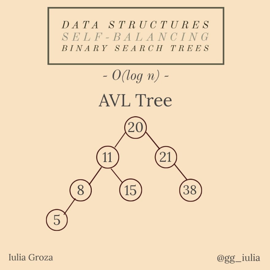
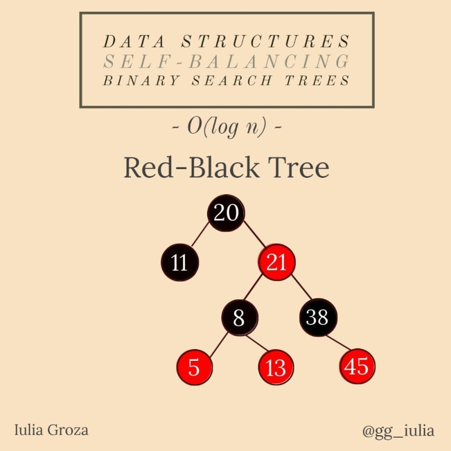
9. Self-balancing trees
All these types of trees are self-balancing binary search trees. The difference is in the way they balance their height in logarithmic time.
AVL Trees are self-balancing after every insertion/deletion because the difference in module between the heights of the left subtree and the right subtree of a node is maximum 1. AVLs are named after their inventors: Adelson-Velsky and Landis.
In Red-Black Trees, each node stores an extra bit representing color, used to ensure the balance after every insert/delete operation.
In Splay trees, recently accessed nodes can be quickly accesed again, thus the amortized time complexity of any operation is still O(log n).
What are they used for?
An AVL seems to be the best data structure in Database Theory.
RBTs are used to organize pieces of comparable data, such as text fragments or numbers. In the version 8 of Java, HashMaps are implemented using RBTs. Data structures in computational geometry and functional programming are also built with RBTs.
Splay trees are used for caches, memory allocators, garbage collectors, data compression, ropes (replacement of string used for long text strings), in Windows NT (in the virtual memory, networking, and file system code).
Properties
the amortized time complexity of ANY operation in ANY self-balancing BST is O(log n);
the maximum height of an AVL in worst case is 1.44 * log2n (Why? *hint: think about the case of an AVL with all levels full, except the last one that has only a single element);
AVLs are the fastest in practice for searching elements, but the rotation of subtrees for self-balancing is costly;
meanwhile, RBTs provide faster insertions and deletions because there are no rotations;
Splay trees don’t need to store any bookkeeping data.
Useful Links
GeeksforGeeks: Red-Black Trees
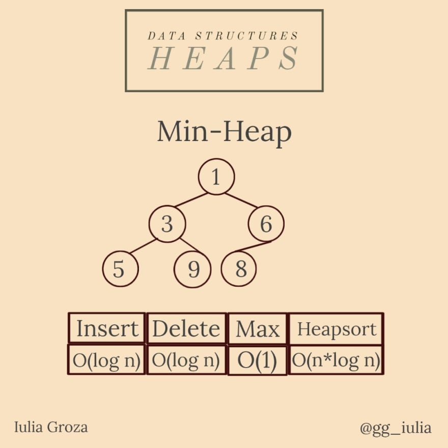
10.Heaps
A min-heap is a binary tree where each node has the property that its value is bigger or equal to its parent’s value: val[par[x]] <= val[x], with x a node of the heap, where val[x] is its value and par[x] its parent.
There is also a max-heap which implements the opposite relation.
A binary heap is a complete binary tree (all its levels are filled, except maybe for the last level).
What are they used for?
As we’ve discussed about it a few days earlier, priority queues can be efficiently implemented using a binary heap because it supports insert(), delete(), extractMax() and decreaseKey() operations in O(log n) time. That way, heaps are also essential in graph algorithms (because of the priority queue).
Anytime that you would need quick access to the maximum/minimum item, a heap is the best option.
Heaps are also the base of the heapsort algorithm.
Properties
it is always balanced: anytime we delete/insert an element in the structure, we just have to “sift”/”percolate” it until it is in the right position;
the parent of a node k > 1 is [k/2] (where [x] is the integer part of x) and its children are 2*kand 2*k+1;
an alternative of a priority queue are set, ordered_map (in C++) or any other ordered structure that can easily permit the access to the minimum/maximum element;
the root is prioritized, so the time complexity of its access is O(1), insertion/deletion are done in O(log n); creating a heap is done in O(n); heapsort in O(n*log n).
Useful Links
11.Tries
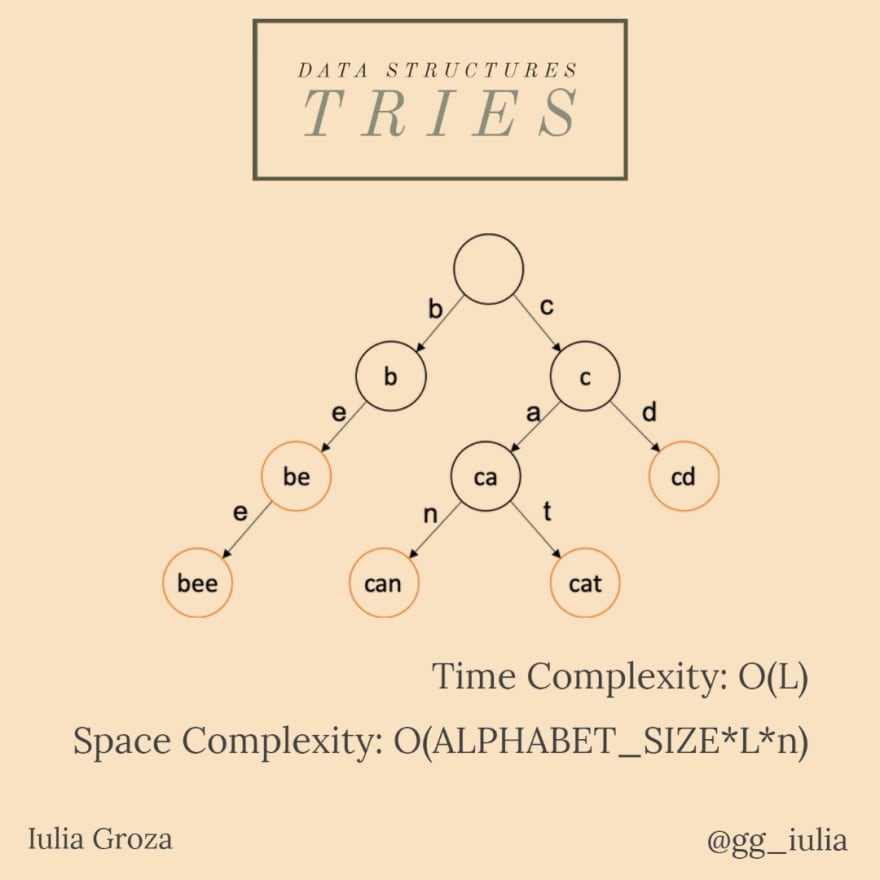
A trie is an efficient information reTRIEval data structure. Also known as a prefix tree, it is a search tree which allows insertion and searching in O(L) time complexity, where L is the length of the key.
If we store keys in a well balanced BST, it will need time proportional to L * log n, where n is the number of keys in the tree. That way, a trie is a way faster data structure (with O(L)) compared to a BST, but the penalty is on the trie storage requirements.
What are they used for?
A trie is mostly used for storing strings and their values. One of its coolest application is the typing autocomplete & autosuggestions in the Google search bar. A trie is the best choice because it is the fastest option: a faster search is more valuable than the storage saved if we didn’t use a trie.
Ortographical autocorrection of typed words is also done using a trie, by looking for the word in the dictionary or maybe for other instances of it in the same text.
Properties
it has a key-value association; the key is usually a word or a prefix of it, but it can be any ordered list;
the root has an empty string as a key;
the length difference between a node’s value and its children’s values is 1; that way, the root’s children will store a value of length 1; as a conclusion, we can say that a node x from a level k has a value of length k;
as we’ve said, the time complexity of insert/search operations is O(L), where L is the length of the key, which is way faster than a BST’s O(log n), but comparable to a hashtable;
space complexity is actually a disadvantage: O(ALPHABET_SIZE*L*n).
Useful Links
Medium: Trying to understand tries
12. Segment Trees
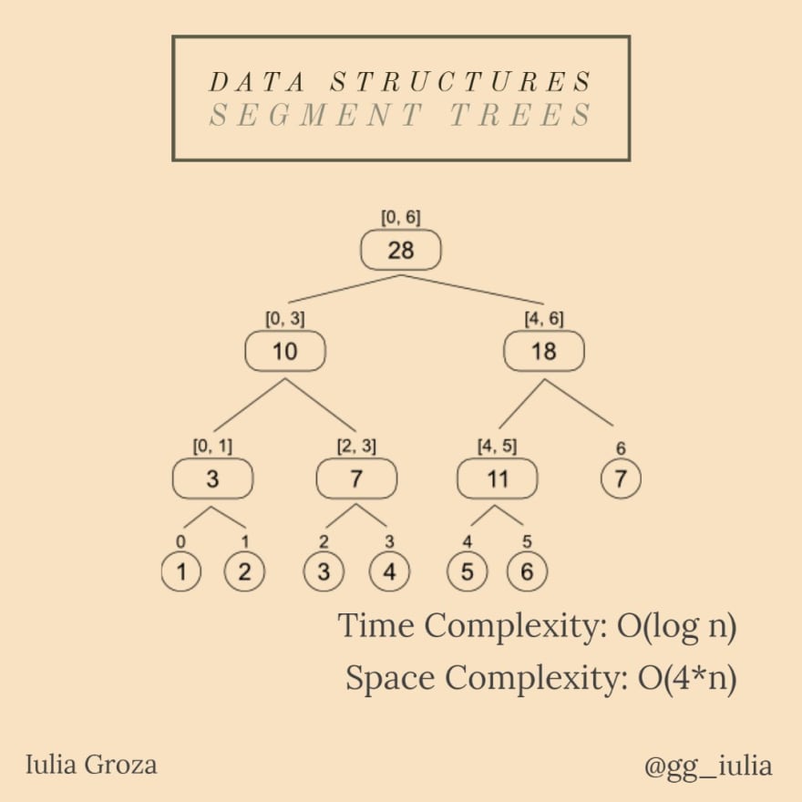
A segment tree is a full binary tree that allows answering to queries efficiently, while still easily modifying its elements.
Each element on index i in the given array represents a leaf labeled with the [i, i] interval. A node having its children labeled [x, y], respectively [y, z], will have the [x, z] interval as a label. Therefore, given n elements (0-indexed), the root of the segment tree will be labeled with [0, n-1].
What are they used for?
They are extremely useful in tasks that can be solved using Divide & Conquer (first Algorithms concept that we are going to discuss) and also might require updates on their elements. That way, while updating the element, any interval containing it is also modified, thus the complexity is logarithmic. For instance, the sum/maximum/minimum of n given elements are the most common applications of segment trees. Binary search can also use a segment tree if element updates are ocurring.
Properties
being a binary tree, a node x will have 2*x and 2*x+1 as children and [x/2] as a parent, where [x] is the integer part of x;
one efficient method of updating a whole range in a segment tree is called “Lazy Propagation” and it is also done in O(log n) (see links below for the implementation of the operations);
they can be k-dimensional : for example, having q queries of finding the sum of given submatrices of one matrix, we can use a 2-dimensional segment tree;
updating elements/ranges require O(log n) time; answering to a query is constant (O(1));
the space complexity is linear, which is a BIG advantage: O(4*n).
Useful Links
CP Agorithms: Segment Trees. Lazy propagation
13. Fenwick Trees
A fenwick tree, also known as a binary indexed tree (BIT), is a data structure that is also used for efficient updates and queries. Compared to Segment Trees, BITs require less space and are easier to implement.
What are they used for?
BITs are used to calculate prefix sums — the prefix sum of the element on the ith position is the sum of the elements from the first position to the ith. They are represented using an array, where every index is represented in the binary system. For instance, an index 10 is equivalent to an index 2 in the decimal system.
Properties
the construction of the tree is the most interesting part: firstly, the array should be 1-indexed; to find the parent of the node x, you should convert its index x to the binary system and flip the right-most significant bit; ex. the parent of node 6 is 4; 6 = 1*2²+1*2¹+0*2⁰ => 1"1"0 (flip)=> 100 = 1*2²+0*2¹+0*2⁰ = 4;
finally, ANDing elements, each node should contain an interval that can be added to the prefix sum (more about the construction and implementation in the links below);
the time complexity is still O(log n) for updates and O(1) on queries, but the space complexity is even a greater advantage: O(n), compared to segment tree’s O(4*n).
Useful Links
14. Disjoint Set Union
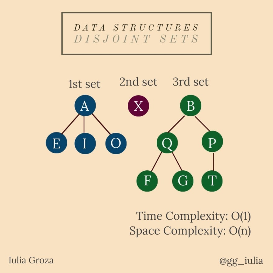
We are given n elements, each of them representing a separate set. Disjoint Set Union (DSU) permits us to do two operations:
UNION — combine any two sets (or unify the sets of two different elements if they’re not from the same set);
FIND — find the set an element comes from.
What are they used for?
DSUs are very important in graph theory. You could check if two vertices come from the same connected component or maybe even unify two connected components.
Let’s take the example of cities and towns. Since neighbour cities with demographical and economical growth are expanding, they can easily create a metropolis. Therefore, two cities are combined and their residents live in the same metropolis. We can also check what city a person lives in, by calling the FIND function.
Properties
they are represented using trees; once two sets are combined, one of the two roots becomes the main root and the parent of the other root is one of the other tree’s leaves;
one kind of practical optimization is the compression of trees by their height; that way, the union is made by the biggest tree to easily update both of their data (see implementation below);
all operations are done in O(1) time.
Useful links
15. Minimum Spanning Trees
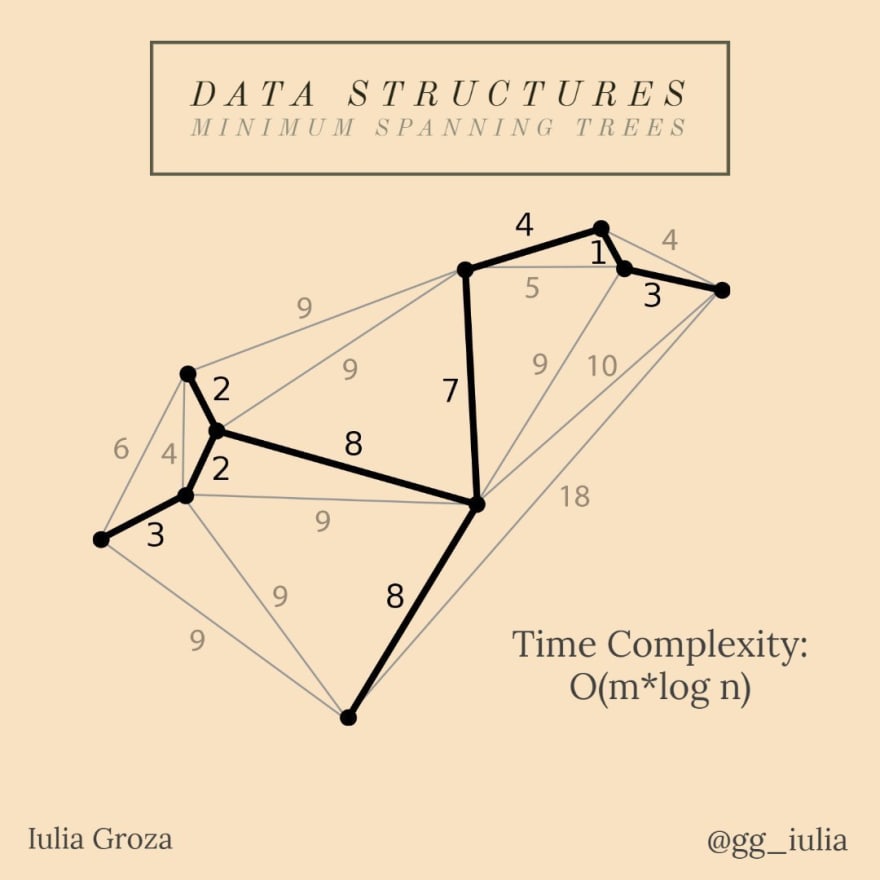
Given a connected and undirected graph, a spanning tree of that graph is a subgraph that is a tree and connects all the nodes together. A single graph can have many different spanning trees. A minimum spanning tree (MST) for a weighted, connected and undirected graph is a spanning tree with weight (cost) less than or equal to the weight of every other spanning tree. The weight of a spanning tree is the sum of weights given to each edge of the spanning tree.
What are they used for?
The MST problem is an optimization problem, a minimum cost problem. Having a network of routes, we can consider that one of the factors that influence the establishment of a national route between n cities is the minimum distance between two adjacent cities.
That way, the national route is represented by the MST of the roads network’s graph.
Properties
being a tree, an MST of a graph with n vertices has n-1 edges; it can be solved using:
* Prim’s Algorithm — best option for dense graphs (graphs with n nodes and the number of edges is close to n(n-1)/2);
* Kruskal’s Algorithm — mostly used; it is a Greedy algorithm based on Disjoint Set Union (we are going to discuss about it too);
the time complexity of building it is O(n log n) or O(n log m) for Kruskal (it depends on the graph) and O(n²) for Prim.
Useful Links
II. Algorithms
1. Divide and Conquer
Divide and Conquer (DAC) is not a specific algorithm itself, but an important category of algorithms that needs to be understood before diving into other topics. It is used to solve problems that can be divided into subproblems that are similar to the original problem, but smaller in size. DAC then recursively solves them and finally merges the results to find the solution of the problem.
It has three stages:
Divide — the problems into subproblems;
Conquer — the subproblems by using recursion;
Merge — the subproblems’ results into the final solution.
What is it used for?
One practical application of DAC is parallel programming using multiple processors, so the subproblems are executed on different machines.
DAC is the base of many algorithms such as Quick Sort, Merge Sort, Binary Search or fast multiplication algorithms.
Properties
each DAC problem can be written as a recurrence relation; so, it is essential to find the basic case that stops the recursion;
its complexity is T(n)=D(n)+C(n)+M(n), meaning that every stage has a different complexity depending on the problem.
Useful Links
Divide and Conquer Implementation
2. Sorting Algorithms
A sorting algorithm is used to rearrange given elements (from an array or list) according to a comparison operator on the elements. When we refer to a sorted array, we usually think of ascending order (the comparison operator is ‘<’). There are various types of sorting, with different time and space complexities. Some of them are comparison based, others not. Here are the most popular/efficient sorting methods:
Bubble Sort
Bubble Sort is one of the simplest sorting algorithms. It is based on a repeated swap between adjacent elements if they are in wrong order. It is stable, its time complexity is O(n²) and it needs O(1) auxiliary space.
Counting Sort
Counting Sort is not a comparison based sorting. It is basically using the frequency of each element (a kind of hashing), determining the minimum and maximum value and then iterating between them to place each element based on its frequency. It’s done in O(n) and the space is proportional to the range of data. It is efficient if the range of input is not significantly greater than the number of elements.
Quick Sort
Quick Sort is an application of Divide and Conquer. It is based on choosing an element as a pivot (first, last or median) and then swapping elements in order to place the pivot between all the elements smaller than it and all the elements bigger than it. It has no additional space and O(n*log n) time complexity — the best complexity for comparison based methods.
Here is a demo with choosing the pivot as the last element:
Merge Sort
Merge Sort is also a Divide & Conquer application. It divides the array in two halves, sorts each half and then merges them. Its time complexity is also O(n*log n), so it is also super fast like Quick Sort, but it unfortunately needs O(n) additional space to store two subarrays at the same time and, finally, merge them.
Radix Sort
Radix Sort uses Counting Sort as a subroutine, so it is not a comparison based algorithm. How do we know CS is not enough? Suppose we have to sort elements in [1, n²]. Using CS, it would take us O(n²). We need a linear algorithm — O(n+k), where elements are in range [1, k]. It sorts the elements digit by digit starting with the least significant one (units), to the most (tens, hundreds etc.). Additional space (from CS): O(n).
Useful Links
3. Searching Algorithms
Searching Algorithms are designed to check for the existence of an element in a data structure and even return it. There are a couple of searching methods, but here are the most popular two:
Linear Search
This algorithm’s approach is very simple: you start searching for your value from the first index of the data structure. You compare them one by one until your value and your current element are equal. If that specific value is not in the DS, return -1.
Time Complexity: O(n)
Binary Search
BS is one efficient search algorithm based on Divide and Conquer. Unfortunately, it only works only on sorted data structures. Being a DAC method, you continuously divide the DS in two halves and compare your in-search value with the middle element’s value. If they are equal, the search is finished. Either way, if your value is bigger/smaller than it, the search should continue on the right/left half.
Time Complexity: O(log n)
Useful Links
4. Sieve of Eratosthenes
Given an integer number n, print all the prime numbers smaller or equal to n.
Sieve of Eratosthenes is one of the most efficient algorithms that solves this problem and it perfectly works for n smaller than 10.000.000.
The method uses a frequency list/map that marks the primality of every number in the range [0, n]: ok[x]=0 if x is prime, ok[x]=1 otherwise.
We begin choosing every prime number from our list and marking its multiples from the list with 1 — that way, we choose the unmarked (0) numbers. Finally, we can easily answer in O(1) to as many queries as we want.
The classical algorithm is essential in many applications, but there are a few optimizations we can make. Firstly, we can easily notice 2 is the only even prime number, so we can check for its multiples separately and then iterate in the range in order to find prime numbers from two to two. Secondly, it is obvious that for a number x, we had previously checked 2x, 3x, 4x etc. when we were iterating through 2, 3 etc. That way, our multiples check for-loop can start from x² every time. Finally, even half of these multiples are even and we are also iterating through odd prime numbers, so we can easily iterate just from 2*x to 2*x in the multiples check loop.
Space complexity: O(n)
Time complexity: O(n*log(log n)) for the classical algorithm, O(n) for the optimized one.
Why O(n*log(log n))?
The answer
Useful Links
Sieve of Eratosthenes Implementation
5. Knuth-Morris-Pratt Algorithm
Given a text of length n and a pattern of length m, find all the occurrences of the pattern in the text.
Knuth-Morris-Pratt Algorithm (KMP) is an efficient way to solve the pattern matching problem.
The naive solution is based on using a “sliding window”, where we compare character to character every time we set a new beginning index, starting from index 0 of the text to index n-m. That way, time complexity is O(m*(n-m+1))~O(n*m).
KMP is an optimization to the naive solution: it is done in O(n) and it is working the best when the pattern has many repeating subpatterns. Thereby, it is also using a sliding window, but instead of comparing all the characters to the substring’s, it is constantly looking for the longest suffix of the current subpattern which is also its prefix. In other words, anytime we detect a mismatch after some matches, we already know some of the characters in the text of the next window. Therefore, it is useless to match them again, so we restart the matching with the same character in the text with a character after that prefix. How do we know how many characters we should skip? Well, we should build a pre-process array that tells us how many characters should be skipped.
Useful Links
6. Greedy
The Greedy method is mostly used for problems that require optimization and the local optimal solution leads to the global optimal solution.
That being said, when using Greedy, the optimal solution at each step leads to the overall optimal solution. However, in most cases, the decision we make at one step affects the list of decisions for the next step. In this case, the algorithm must be mathematically demonstrated. Greedy also produces great solutions on some mathematical problems, but not on all (it is possible that the most optimal solution is not guaranteed)!
A Greedy algorithm generally has five components:
a candidate set — from which a solution is created;
a selection function — chooses the best candidate;
a feasibility function — can determine if a candidate is able to contribute to the solution;
an objective function — assigns the candidate to the (partial) solution;
a solution function — builts the solution from the partial solutions.
Fractional Knapsack Problem
Given weights and values of n items, we need to put these items in a knapsack of capacity W to get the maximum total value in the knapsack (taking pieces of items is allowed: the value of a piece is proportional with its weight).
The basic idea of the greedy approach is to sort all the items on basis of their value/weight ratio. Then, we can add as many whole items as we can. In the moment we find an item heavier (w2) than our available weight left in the knapsack (w1), we will fractionate it: take only w2-w1 of it to maximize our profit. It is guaranteed this greedy solution is correct.
Useful links
Maximum number of non-overlapping intervals Implementation
Fractional Knapsack Problem Implementation
7. Dynamic Programming
Dynamic Programming (DP) is a similar approach to Divide & Conquer. It also breaks the problem into similar subproblems, but they are actually overlapping and codependent — they’re not solved independently.
Each subproblem’s result can be used anytime later and it is built using memoization (precalculation). DP is mostly used for (time & space) optimization and it is based on finding a recurrence.
DP applications include Fibonacci number series, Tower of Hanoi, Roy-Floyd-Warshall, Dijkstra etc. Below we are going to discuss about a DP solution of the 0–1 Knapsack Problem.
0–1 Knapsack Problem
Given weights and values of n items,we need to put these items in a knapsack of capacity W to get the maximum total value in the knapsack (fractioning items just as in the Greedy solution is not allowed).
The 0–1 property is given by the fact that we should either pick the whole item or not choose it at all.
We build a DP structure as a matrix dp[i][cw]storing the maximum profit that we can obtain by choosing i objects whose total weight is cw. It is easy to notice that we should firstly initialize dp[1][w[i]] with v[i], where w[i] is the weight of the ith object and v[i] its value.
The recurrence is the following: dp[i][cw] = max(dp[i-1][cw], dp[i-1][cw-w[i]]+v[i]). Let’s analyze it a little bit.
dp[i-1][cw] depicts the case in which we do not add the current item in the knapsack. dp[i-1][cw-w[i]]+v[i] is the case in which we add the item. That being said, dp[i-1][cw-w[i]] is the maximum profit of taking i-1 elements: so their weight is the current weight without our item’s weight. Finally, we add our item’s value to it.
The answer is stored into dp[n][W]. An optimization is made with a simple observation: in the recurrence, the current line (row) is influenced only by the previous line. Therefore, storing the DP structure into a matrix is unnecessary, so we should choose an array for a better space complexity: O(n). Time complexity: O(n*W).
Useful Links
0–1 Knapsack Problem Implementation
8. Longest Common Subsequence
Given two sequences, find the length of the longest subsequence present in both of them. A subsequence is a sequence that appears in the same relative order, but not necessarily contiguous. For example, “bcd”, “abdg”, “c” are subsequences of “abcdefg”.
Here is another application of dynamic programming. The LCS algorithm uses DP in order to solve the problem from above.
The actual subproblem is going to find the longest common subsequence that starts from index i in the sequence A, respectively from index j in the sequence B.
Next, we will build the DP structure lcs[ ][ ](matrix), where lcs[i][j] is the maximum length of a common subsequence that starts from index i in A, respectively index j in B. We are going to build it in a top-down manner. The solution is, obviously, stored in lcs[n][m], where n is the length of A and m the length of B.
The recurrence relation is pretty simple and intuitive. For simplicity, we are going to consider that both sequences are 1-indexed. Firstly, we are going to initialize lcs[i][0], 1<=i<=n, and lcs[0][j], 1<=j<=m, with 0, as basic cases (there is no subsequence that starts from 0). Then, we will take into consideration two main cases: if A[i] is equal to B[j], then lcs[i][j] = lcs[i-1][j-1]+1 (one more identic character than the previous LCS). Otherwise, it will be the maximum between lcs[i-1][j] (if A[i] is not taken into consideration) and lcs[i][j-1] (if B[j] is not taken into consideration).
Time Complexity: O(n*m)
Additional Space: O(n*m)
Useful Links
9. Longest Increasing Subsequence
Given a sequence A of n elements, find the length of the longest subsequence such that all of its elements are sorted in increasing order. A subsequence is a sequence that appears in the same relative order, but not necessarily contiguous. For example “bcd”, “abdg”, “c” are subsequences of “abcdefg”.
LIS is another classic problem that can be solved using Dynamic Programming.
Finding the maximum length of an increasing subsequence is done using an array l[ ] as a DP structure, where l[i] is the maximum length of an increasing subsequence that contains A[i], having its elements from the [A[i], …, A[n]]subsequence. l[i] is 1, if all the elements after A[i]are smaller than it. Otherwise, it’s 1+ maximum between all the elements after A[i] which are bigger than it. Obviously, l[n]=1, where n is the length of A. The implementation is done in a bottom-up manner (starting from the end).
One optimization problem appears in searching the maximum between all the elements after the current element. The best we can do is to binary search the maximum element.
To also find a subsequence of the now known maximum length, we just have to use an additional array ind[ ], that stores the index of each maximal value.
Time Complexity: O(n*log n)
Additional Space: O(n)
Useful Links
10. Convex Hull
Given a set of n points in the same plane, find the minimum area convex polygon that contains all of the given points (situated inside the polygon or on its sides). Such polygon is called a convex hull. The convex hull problem is a classic geometry that has many applications in real life. For instance, collision avoidance: if the convex hull of the car avoids collisions then so does the car. Computation of paths is done using convex representations of cars. Shape analysis is also done with the help of convex hulls. That way, image processing is easily done by matching models by their convex deficiency tree.
There are some algorithms used to find the convex hull, like Jarvis’ Algorithm, Graham scanning etc. Today we are going to discuss about Graham scanning and some useful optimizations.
Graham scanning sorts the points by their polar angle — the slope of the line determined by a certain point and the other chosen points. Then, a stack is used to store the convex hull at the current moment. When a point x is pushed into the stack, other points will be popped out of the stack until x and the line determined by the last two points form an angle smaller than 180°. Finally, the last point introduced into the stack closes the polygon. This approach has a time complexity of O(n*log n) because of sorting. However, this method can produce precision errors when calculating the slope.
One improved solution that has the same time complexity, but smaller errors sorts the points by their coordinates (x, then y). Then we consider the line formed by the leftmost and rightmost points and the problem is divided in two subproblems. Finally, we find the convex hull on each side of the line. The convex hull of all the given points is the reunion of the two hulls.
Useful Links
11. Graph Traversals
The problem of traversing graphs reffers to visiting all the nodes in a particular order, usually computing other useful information along the way.
Breadth-First Search
The Breadth-First Search (BFS) algorithm is one of the most common ways to determine if a graph is connected or not — or, in other words, to find the connected component of the source node of the BFS.
BFS is also used to compute the shortest distance between the source node and all the other nodes. Another version of BFS is Lee’s Algorithm used to compute the shortest path between two cells in a grid.
The algorithm starts by visiting the source node and then its neighbours that will be pushed into a queue. The first element from the queue is popped. We will visit all of its neighbours and push the ones that were not previously visited into the queue. The process is repeated until the queue is empty. When the queue becomes empty, it means that all the reachable vertices have been visited and the algorithm ends.
Depth-First Search
The Depth-First Search (DFS) algorithm is another common traversal method. It is actually the best option when it comes to checking the connectivity of a graph.
First, we visit the root node and push it into a stack. While the stack is not empty, we examine the node at the top. if the node has unvisited neighbours, one of them is chosen and pushed in the stack. Otherwise, if all of its neighbours had been visited, we pop the node. When the stack becomes empty, the algorithm ends.
After such traversal, a DFS tree is formed. The DFS tree has many applications; one of the most common is storing the “starting” and “ending” time of each node — the moment it enters the stack, respectively the moment it is popped out from it.
Useful Links
12. Floyd-Warshall Algorithm
The Floyd-Warshall / Roy-Floyd Algorithm solves the All Pairs Shortest Path problem: find the shortest distances between every pair of vertices in a given edge-weighted directed graph.
FW is a Dynamic Programming application. The DP structure (matrix) dist[ ][ ] is initialized with the input graph matrix. Then we consider each vertex as an intermediate between other two nodes. The shortest paths are updated between every two pair of nodes, with any node k as an intermediate vertex. If k is an intermediate in the sortest path between i and j, dist[i][j] becomes the maximum between dist[i][k]+dist[k][j] and dist[i][j].
Time Complexity: O(n³)
Space Complexity: O(n²)
Useful Links
13. Dijkstra’s Algorithm & Bellman-Ford Algorithm
Dijkstra’s Algorithm
Given a graph and a source vertex in the graph, find the shortest paths from the source to all vertices in the given graph.
Dijkstra’s Algorithm is used to find such paths in a weighted graph, where all weights are positive.
Dijkstra is a Greedy algorithm that uses a shortest path tree (SPT) with the source node as the root. A SPT is a self-balancing binary tree, but the algorithm can be implemented using a heap (or a priority queue). We’re going to discuss about the heap solution, because its time complexity is O(|E|*log |V|). The idea is to work with an adjacency list representation of the graph. That way, the nodes will be traversed in O(|V|+|E|) time using BFS.
All vertices are traversed with BFS and those for which the shortest distance is not finalized yet are stored into a Min-Heap (priority queue).
The Min-Heap is created and every node is pushed into it along with their distance values. Then, the source becomes the root of the heap with a distance of 0. The other nodes will have infinite assigned as a distance. While the heap’s not empty, we extract the minimum distance value node x. For every vertex y adjacent to x, we check if y is in the Min-Heap. In this case, if the distance value is bigger than the weight of (x, y) plus distance value of x, then we update the distance value of y.
Bellman-Ford Algorithm
As we’ve previously said, Dijkstra works only on positively weighted graphs. Bellman solves this problem. Given a weighted graph, we can check if it contains a negative cycle. If not, then we can also find the minimum distances from our source to the others (negative weights possible).
Bellman-Ford suites well for distributed systems, although its time complexity is O(|V||E|).
We initialize a dist[ ] just like in Dijkstra. For *|V|-1times, for each (x, y) edge, if dist[y] > dist[x] + weight of (x, y), then we update dist[y] with it.
We repeat the last step to possibly find a negative cycle. The idea is that the last step guarantees the minimum distance if there is no negative cycle. If there is any node that has a shorter distance in the current step than in the last one, then a negative cycle was detected.
Useful Links
14. Kruskal’s Algorithm
We have previously discussed about what a Minimum Spanning Tree is.
There are two algorithms that find the MST of a graph: Prim (useful for dense graphs) and Kruskal (ideal for most graphs). Now we are going to discuss about Kruskal’s Algorithm.
Kruskal has developed a greedy algorithm in order to find an MST. It’s efficient on rare graphs, because its time complexity is O(|E|*log |V|).
The algorithm’s approach is the following: we sort all the edges in increasing order of their weight. Then, the smallest edge is picked. If it does not form a cycle with the current MST, we include it. Otherwise, discard it. The last step is repeated until there are |V|-1 edges in the MST.
The inclusion of edges into the MST is done using Disjoint-Set-Union, also previously discussed.
Useful Links
15. Topological Sorting
A Directed Acyclic Graph (DAG) is simply a directed graph which contains no cycles.
Topological sorting in a DAG is a linear ordering of vertices such that for every arch (x, y), node x comes before node y.
Obviously, the first vertex in a topological sorting is a vertex with a 0 in-degree (there are no arches directing to it).
Another special property is that a DAG doesn’t have a unique topological sorting.
The BFS implementation follows this routine: a node with a 0 in-degree is found and pushed the first into the sorting. This vertex is removed from the graph. As the new graph is also a DAG, we can repeat the process.
At any point during DFS, a node can be in one of these three categories:
nodes that we finished visiting (popped from the stack);
nodes that are currently on the stack;
nodes that are yet to be discovered.
If during DFS in a DAG a node x has an outgoing edge to a node y, then y is either in the first or the third category. If y was on the stack, then (x, y) would end a cycle, fact that contradicts the DAG definition.
This property actually tells us that a vertex is popped from the stack after all of its outgoing neighbours are popped. So to topological sort a graph, we need to keep track of a reversed order list of the popped vertices.
Useful Links
Topological Sorting Implementation
Woah, you have made it to the end of the article. Thanks for your attention! :) Have fun coding!




This comment has been removed by a blog administrator.
ReplyDeleteNice Blog information about Hacking Services. Sometimes hacking is boon for us and it can be change to the Modern Technology, The real Hackers can resolve your most critical and technical problem and issues without any difficulty. If you are really searching professional hackers to resolving the technical issues then you can visit at All Tech Facts and grab the latest information about latest Technologies.
ReplyDelete